Recommender Systems and Collaborative Filtering - Walkthrough
This is a walkthrough of Collaborative Filtering that I wrote for a class.
Summary
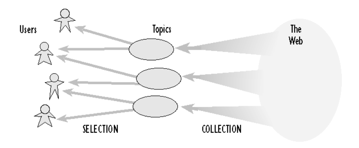
Every user on the internet today is faced with an overwhelming set of choices on almost every website he/she visits. Be it Facebook, Spotify, Amazon or Google, there is a need to filter, rank and deliver relevant information quickly in order to alleviate the problem of information overload. Recommender systems are used in almost every major website these days to solve this problem by searching through a large volume of dynamically generated information to provide users with personalized content and services. See Figure 1 1.
After completing this walkthrough you should be able to :
-
Understand what Recommender Systems do.
-
Get a high level overview of different approaches used in Recommender Systems.
-
Understand the concept of collaborative filtering.
-
Learn how to implement collaborative filtering using low dimensional matrix factorization method.
-
Get a hands on experience on building a collaborative filtering recommender system for a real-life dataset.
Background
Recommender systems have become extremely popular in recent years. They
are a subclass of information filtering systems that seek to predict the
“rating” or “preference” that a user would give to an item. Applications
of recommender systems include: movies, music, news, books, research
articles, search queries, social tags, and products. For example,
recommending news articles to on-line newspaper readers.
Basic Concepts :
User: any individual who provides ratings to a system. User who
provides provides ratings ratings and user who receive receive
recommendations recommendations.
Item: anything for which a human can provide a rating. Eg. art,
books, CDs, journal articles, music, movie, or vacation destinations
Ratings: vote from a user for an item by means of some value.
Scalar/ordinal ratings (5 points Likert scale), binary ratings
like/dislike), unary rating (observed/abase of rating).
Recommender systems typically produce a list of recommendations in one of two ways – through collaborative and content-based filtering.
-
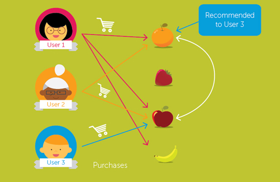
Collaborative filtering: This approach is used to build a model from user’s past behaviour i.e. items previously purchased or selected and/or numerical ratings given to those items as well as similar decisions made by other users. This model is then used to predict items (or ratings for items) that the user may have an interest in.
-
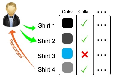
Content-based filtering: This approach uses features of an item in order to recommend additional items with similar features/properties.
Sometimes the above two approaches are often combined and termed as Hybrid Recommender Systems.


The differences between collaborative and content-based filtering can be
demonstrated by comparing two popular music recommender systems –
Last.fm and Pandora Radio.
Last.fm creates a “station” of recommended songs by observing what bands
and individual tracks the user has listened to on a regular basis and
comparing those against the listening behavior of other users. Last.fm
will play tracks that do not appear in the user’s library, but are often
played by other users with similar interests. As this approach leverages
the behavior of users, it is an example of a collaborative filtering
technique.
Pandora uses the properties of a song or artist (a subset of the 400
attributes provided by the Music Genome Project) in order to seed a
“station” that plays music with similar properties. User feedback is
used to refine the station’s results, deemphasizing certain attributes
when a user “dislikes” a particular song and emphasizing other
attributes when a user “likes” a song. This is an example of a
content-based approach.
Each type of system has its own strengths and weaknesses. In the above
example, Last.fm requires a large amount of information on a user in
order to make accurate recommendations. This is an example of the cold
start problem, and is common in collaborative filtering systems. While
Pandora needs very little information to get started, it is far more
limited in scope (for example, it can only make recommendations that are
similar to the original seed).
Recommender systems are a useful alternative to search algorithms since they help users discover items they might not have found by themselves. Interestingly enough, recommender systems are often implemented using search engines indexing non-traditional data.
In this tutorial we will be exploring an implementation of Collaborative Filtering using matrix factorization.
The Problem
To illustrate an everyday application of Collaborative Filtering, let’s
consider building the “Recommended Movies” section of IMDB. Most of the
recommender systems usually have a set of users and a group of items,
such as videos, movies, books or music. A common insight that these
recommenders follow are that personal tastes are correlated. If Alice
and Bob both like X and Alice likes Y then Bob is more likely to like Y
especially (perhaps) if Bob knows Alice. Thus, given that the users have
rated some items in the system, we would like to predict how the users
would rate the items that they have not yet rated, so that we can make
recommendations to the users.
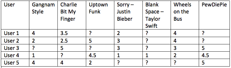
Assume each user gives a movie a rating between 1 and 5 stars and we
have 5 users and 7 movies. We can represent this users and video ratings
information as a matrix such as the one in figure .
Our task now is to predict the ratings for all the entries with ?. We
will use low dimensional matrix factorization method to accomplish this.
Low Dimensional Matrix Factorization
To get the intution behind matrix factorization, lets consider the
example in figure. As discussed above personal tastes
are correlated. For example, two users would give high ratings to a
certain movie like the actors/singers of the video or if the genre is
liked by both the users. Hence, if we can find these
characteristics/features/properties of users and movies, we can easily
predict the rating of unknown movies. Also the number of features are
very small as compared to number of users and movies. Now lets see the
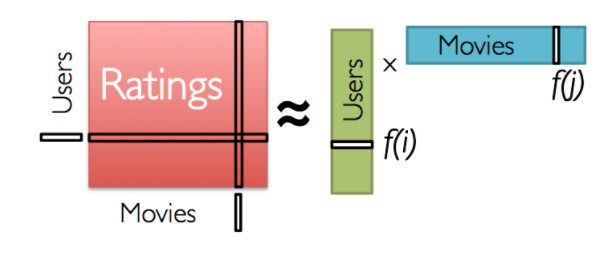
math behind matrix factorization. We need to obtain the two matrices:
users(P) and movies(Q)
We have a \(m \times n\) matrix of users and items and we need to find two
matrices P(\(m \times k\)) and Q(\(n \times k\)) such that their product
approximates R. See Figure below. Note:
\(k \ll m,n\) \(R \approx P \times Q^T = \widehat{R}\)
Why not SVD?
You must be wondering why we are not using SVD for factorization. The
problem is that SVD is not defined if there are missing values in
matrix. We can tackle this problem by filling missing values with zeros
or the average rating that user has given to rest of the videos. But if
the matrix is too big, millions of users and items then this may not be
a good idea.
Cold Start
A common problem faced by most recommender systems is something called
as a Cold start problem.
In collaborative filtering, the recommender system tries to infer the
rating an active user would give to an item from the choices like-minded
users would have made. This approach would fail when there are some
items which no user has rated previously. Specifically, it concerns the
issue that the system cannot draw any inferences for users or items
about which it has not yet gathered sufficient information.
Gradient Descent
How do we now find the matrices P and Q? The idea
behind finding the values for these two matrices is that their products
should nearly be the same as the one in figure above along with
the predicted values for the missing values.
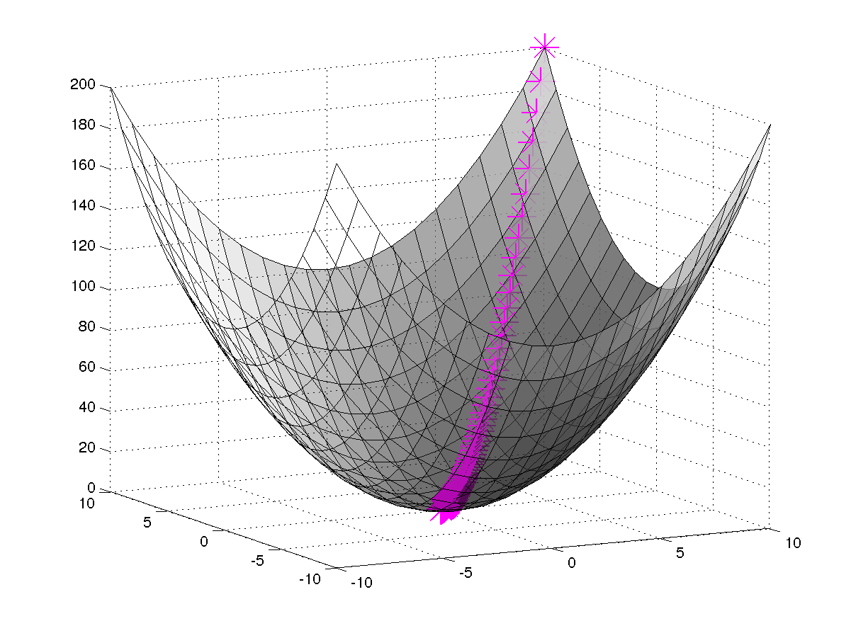
To do this, we can start off by initializing P and Q
with random values and use gradient descent to find the local minima of
the difference between the actual matrix and the calculated matrix
iteratively.
We can write the error between the estimated rating and actual rating
for every user-video pair as given below. Our task here is to minimize
the error in each individual rating.
Note: Objective function is multiplied by a factor of 1/2 in order to
remove 2 during differentiation.
\(e_{ij}^2 = \frac{1}{2}(r_{ij} - \hat{r}_{ij})^2 = \frac{1}{2}(r_{ij} - \sum_{k=1}^K{p_{ik}q_{kj}^T})^2\\\)
Now we need to know the direction in which we should modify the values
of \(p_ik\) and \(q_kj\). This can be obtained by calculating the gradient
at the current value. This is done by differentiating the above equation
with respect to \(p_{ik}\) and \(q_{kj}\) separately :
\(\frac{\partial}{\partial p_{ik}}e_{ij}^2 = -(r_{ij} - \hat{r}_{ij})(q_{kj})\)
\(\frac{\partial}{\partial q_{ik}}e_{ij}^2 = -(r_{ij} - \hat{r}_{ij})(p_{ik})\)
Now we can write the update rule for \(p_{ik}\) and \(q_{kj}\) as follows :
\(p_{ik}^{t+1} = p_{ik}^t - \alpha \frac{\partial}{\partial p_{ik}^t}e_{ij}^2 = p_{ik}^t - \alpha (-r_{ij} + \hat{r}_{ij})q_{kj}^t\)
\(q_{kj}^{t+1} = q_{kj}^t - \alpha \frac{\partial}{\partial q_{kj}^t}e_{ij}^2 = q_{kj}^t - \alpha (-r_{ij} + \hat{r}_{ij})p_{ik}^t\)
Weighted Objective Function
In order to penalize only the known rating we will be using weighted objected function where \(w_{ij} = 1\) if \(r_{ij}\) is observed and \(w_{ij} = 0\) otherwise. \(\min_{P,Q} \frac{1}{2}\times w_{ij}(r_{ij} - \sum_{k=1}^K{p_{ik}q_{kj}^T})^2\)
Regularization
The above algorithm can lead to overfitting. To avoid this, we use L2
regularization to minimize the norm of the residual as follows :
\(e_{ij}^2 = \frac{1}{2}\times w_{ij}(r_{ij} - \sum_{k=1}^K{p_{ik}q_{kj}^T})^2 + \lambda {(||P||^2 + ||Q||^2)}\)
\(\lambda\) provides a knob on the magnitudes of the user-feature and
video-feature vectors. It ensures that P and Q would give a good
approximation of R without having to contain large numbers. Thus our
objective function now becomes:
\(\min_{P,Q} \frac{1}{2}||W\cdot(R-PQ^T)||^2 + \lambda(||P||^2 + ||Q||^2)\)
Here W is the indicator matrix i.e. \(w_{ij} = 1\) if \(r_{ij}\) is observed
and \(w_{ij} = 0\) otherwise.
The new update rules after calculating the
gradient are as follows:
\(\Delta P = W\cdot(PQ^T - R)Q +2\lambda P\)
\(\Delta Q = (W\cdot(PQ^T - R))^TP +2\lambda Q\)
\(P^{t+1} = P^t - \alpha \Delta P^t = P^t - \alpha(W\cdot(P^tQ^{T,t} - R)Q^t +\lambda P^t)\)
\(Q^{t+1} = Q^t - \alpha \Delta Q^t = Q^t - \alpha((W\cdot(P^tQ^{T,t} - R))^TP^t +\lambda Q^t)\)
Note: Multiplication factor 2 can be consumed in \(\lambda\).
Biases
The variation in rating values is most of the times associated with either the item being rated or the user who is rating. Certain users consistently give higher ratings to items while sometimes the item always commands a higher rating from all the users. We use a first order approximation of the above bias as follows : \({b_i}_j = \mu + b_i + b_j\) Where \(\mu\) is the overall average rating for the item.
Lab
Now let’s perform a more thorough analysis of collaborative filtering
using matrix factorization method. To do this we will use the dataset
available here : http://grouplens.org/datasets/movielens/100k/
The goal of this exercise is to build a recommendation system for IMDB.
More specifically :
-
Construct the User-Item Matrix.
-
Define a factorization model - cost function. We will use matrix factorization, regularization and gradient descent to obtain a model that minimizes the below function. \(\min_{M,U} \frac{1}{2}||R\cdot(Y - MU^T)||_F^2 + \lambda(||M||_F^2 + ||U||_F^2)\) Here M is the movie matrix, U is the user matrix, R is the indicator weight matrix \(||\cdot||_F\) is Frobenius norm, the operator \(\cdot\) means the dot product and $\lambda$ is the regularization parameter.
-
Understand the impact of increasing or decreasing the number of features on the accuracy of the model.
-
Experiment the convergence of the model by varying the learning rate and the regularization parameters.
-
Understand the impact of adding bias.
Load the dataset
Download the dataset from this link
http://pages.cs.wisc.edu/~ashenoy/CS532/ Since the above dataset has
many files and asks you to merge the files using specific commands we
have merged the data for you and have created training and testing
datasets. The dataset in total has 100K ratings. We will be using 80K
for training and 20K for testing. train_all.mat has two matrices
each of size \(1682 \times 943\) matrix. In Rating_train(Y) each
entry (i,j) is the rating given to the ith movie by jth user and
L_train(R) is the corresponding indicator matrix. Similarly
test_all.mat has two matrices each of size $1682 \times 943$
matrix. test_Y represents the corresponding test rating matrix and
test_R as the corresponding test indicator matrix.
Write the MATLAB code to load train_all.mat and test_all.mat
and verify the above.
Initialize learning rate, regularization parameter and maximum number of iterations
Now that the dataset is loaded and we have the training and testing set,
we can now initialize the following tuning parameters :
\(alpha = 0.001
lambda = 10
max\_iter = 500\)
Initialize the M(movies) and U(users) matrix
M and U matrices are the factors of the ratings matrix Y. Let’s start with a feature size of 10 and initialize these two matrices with appropriate dimensions and fill them with normally distributed random values.
Gradient Descent
Now that you have the M(movies) and U(users) matrices, write code to
update M and U using gradient descent method :
\(M^{t+1} = M^t - \alpha(R\cdot(M^tU^{t,T}-Y)U^t +\lambda M^t)\)
\(U^{t+1} = U^t - \alpha((R\cdot(M^tU^{t,T})-Y)^TM^t +\lambda U^t)\)
This has to be performed \(max\_iter\) number of times.
Formulate the loss function
Everytime after updating M and U, write code to check for the
convergence. We can assume convergence if the calculated error using the
formula below is less than a threshold 0.0001. If the convergence
condition is met we should stop the gradient calculation.
\(\frac{||M^{t+1}-M^t||^2_F+||U^{t+1}-U^t||^2_F }{||M^t||^2_F+||U^t||^2_F} < \epsilon\)
Predicted Ratings
After performing all of the above steps, you will end up with an updated M and U matrix. Lets call them \(M\_result\) and \(U\_result\) and assign them to these two new variables. Now we can obtain the predicted ratings matrix by calculating the dot product of \(M\_result\) and \(U\_result\).
Calculate Error
Now that you have the predicted ratings matrix, let’s calculate the
error rate using the test dataset.
\(error\_rate = \frac{||test\_R \cdot (predicted\_matrix - test\_Y)||^2_F}{||test\_Y||^2_F}\)
Varying number of features
Now let’s try and analyze how varying the number of features in M and U matrices impacts the accuracy. Plot a graph between \(error\_rate\) on Y axis and \(num\_of\_features\) on X axis. What do you observe? what is the best value of number of features? Take atleast 10 values ranging from min to max number of features.
Varying regularization parameter
Now let’s analyze how varying \(\lambda\) impacts the accuracy. Plot a graph between \(error\_rate\) on Y axis and \(\lambda\) on X axis. What do you observe? what is the best value of lambda? Take logarithmic values of lambda( i.e 0.01, 0.1 etc). Take at least 10 values.
Varying learning rate
Also analyze how varying \(\alpha\) impacts the convergence rate. What happens if you make alpha too small( like 0.0001 or 0.00001), keeping number of iterations as same? Also what if you make alpha too big(like 1, 10)?
Predict missing ratings with best values of parameters
Now that you have tuned all the parameters and have got the best values of each of them, lets find out the missing ratings in Y. Output the result(user, movie, rating) in a text file. Note: use the indicator matrix to find out missing entries and round them before writing in text file.
If you found this work useful please cite as:
@misc{AshishShenoy_Rec_Sys,
  author        = {Shenoy, Ashish},
  title         = {Recommender Systems and Collaborative Filtering - Walkthrough},
  howpublished  = {\url{https://www.ashishvs.in}},
  year          = {2017},
  note          = {Accessed: 2017-03-21},
  url           = {www.ashishvs.in}
}